Using the TemplateSynthesis class
For more general purposes, using SMIETRun is sufficient. However,
for more complicated manipulation, you can use the TemplateSynthesis
module directly. This gives additional flexibility, including:
playing around with different SlicedShowers
analyzing the performance of the synthesis
changing site parameters / frequency ranges
understanding what the code does under the hood
using SlicedShowers as targets
Additionally, this approach is valid with the JAX version, which can be
nice to have a direct comparison with. Here we only show the numpy
version, but replace smiet.numpy -> smiet.jax, and the rest is
the same.
from smiet.numpy import TemplateSynthesis, SlicedShower, CoreasShower, Shower
from smiet import units

import matplotlib.pyplot as plt
import numpy as np
Running a single synthesis between SlicedShowers
# Selections (to be put in main)
ANT_DEBUG = None
FREQ = [30, 500, 100]

# Variables
shower_path = '/home/kwatanabe/Projects/radio-ift/radio_resources/template_synthesis/origin_library/base'
shower_origin = "000900"
shower_target = "000910"
origin = SlicedShower(f'{shower_path}/SIM{shower_origin}.hdf5')
target = SlicedShower(f'{shower_path}/SIM{shower_target}.hdf5')

synthesis = TemplateSynthesis(freq_ar=FREQ)

synthesis.make_template(origin)

total_geo_synth, total_ce_synth = synthesis.map_template(target)

# Get the target trace for comparison
ant_names = synthesis.get_antenna_names()
origin_time = synthesis.get_time_axis()
dt_res = synthesis.delta_t
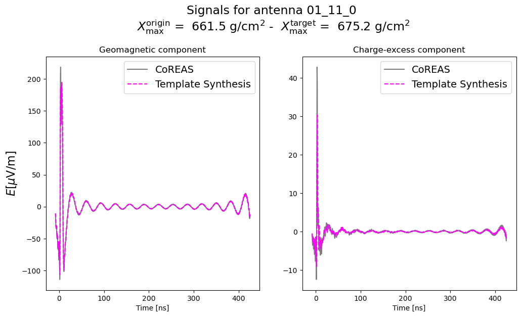
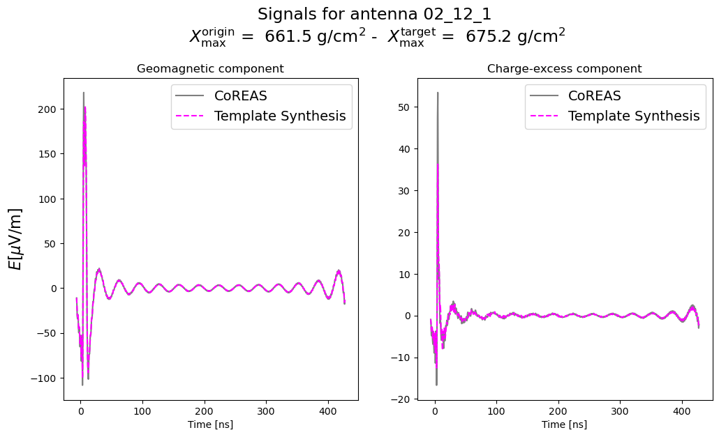
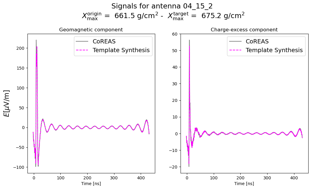
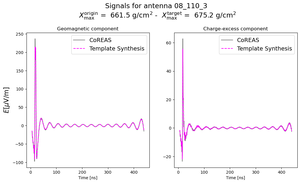
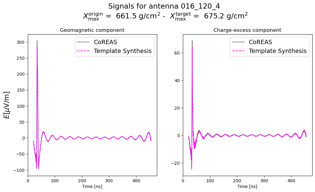
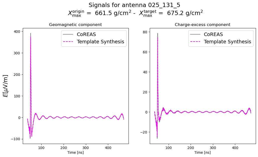
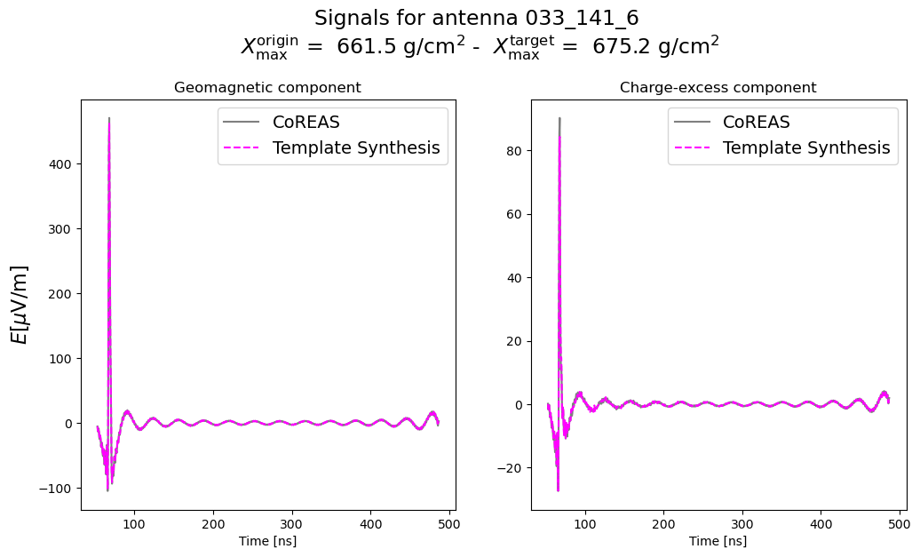
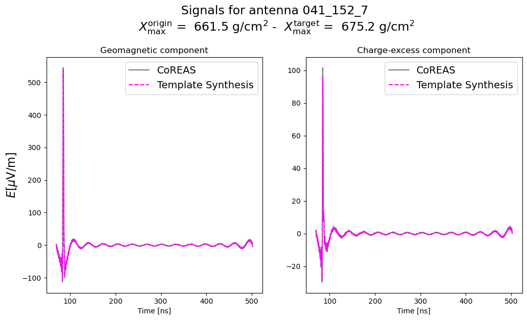
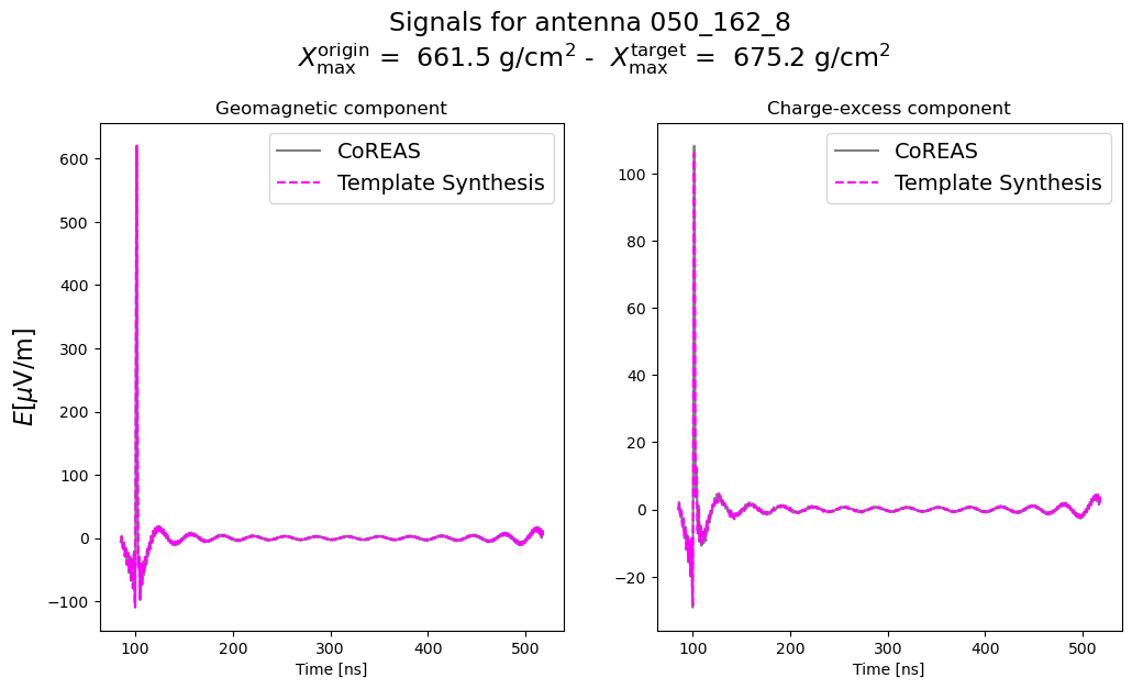
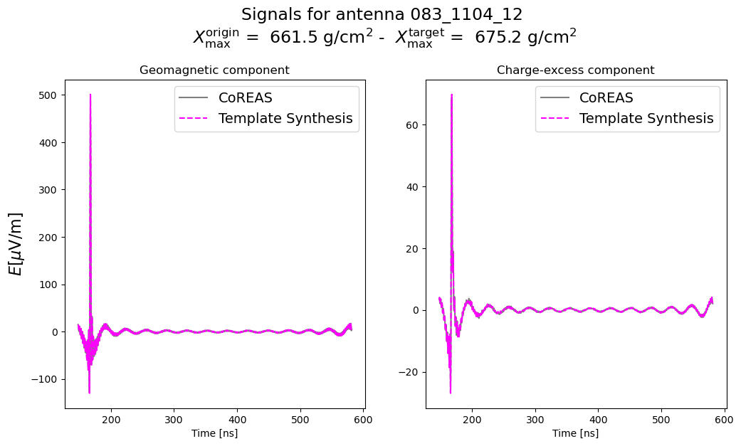
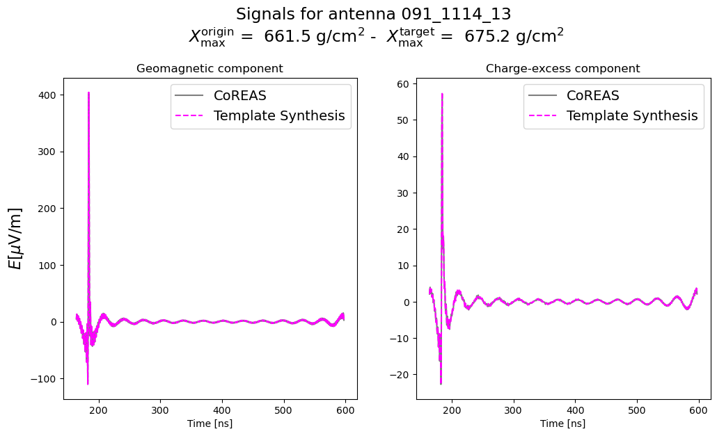
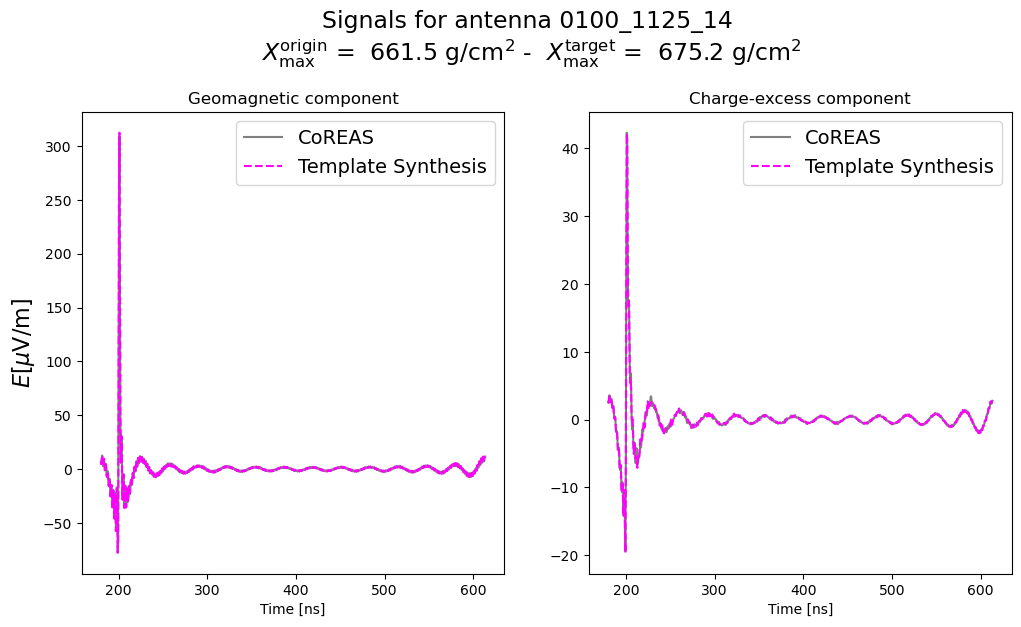
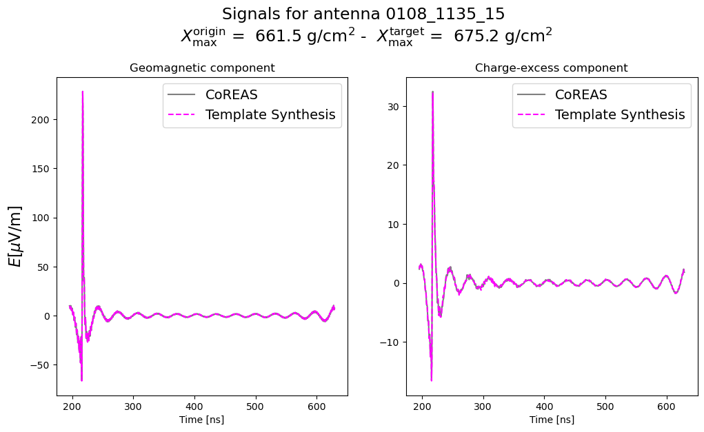
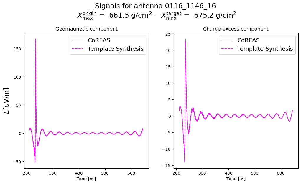
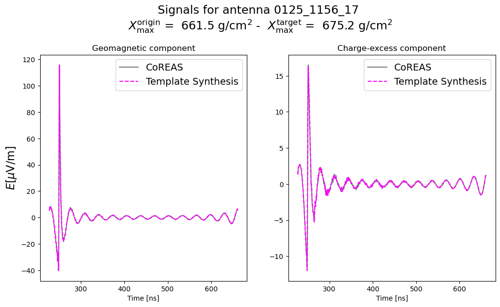
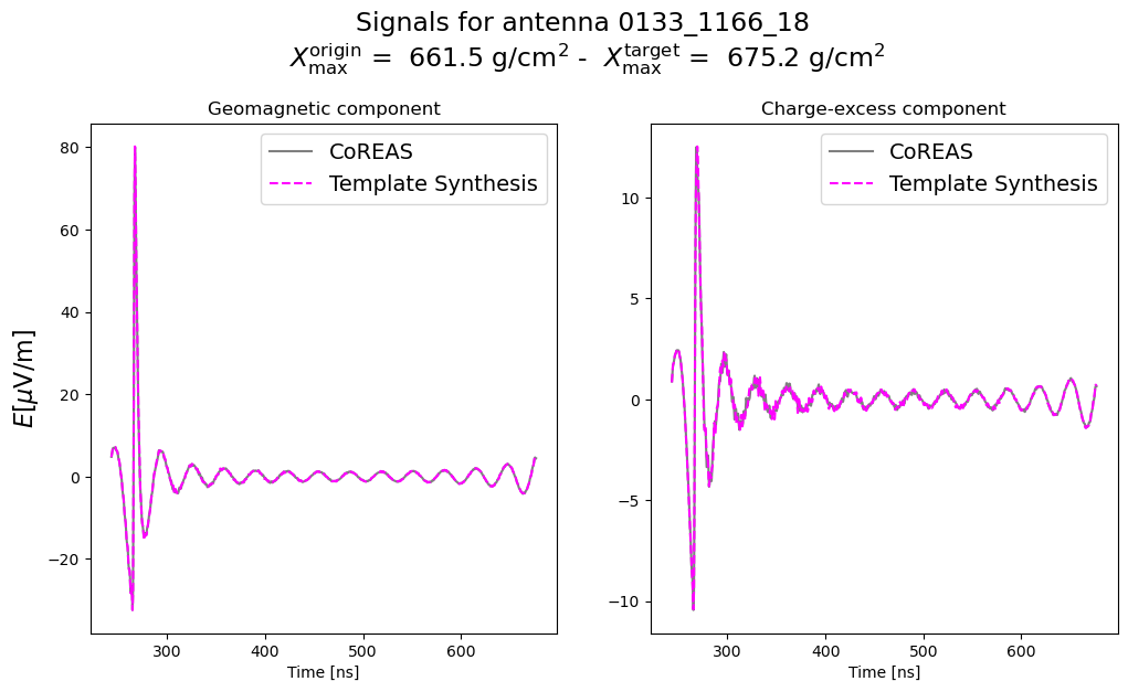
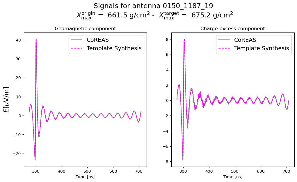
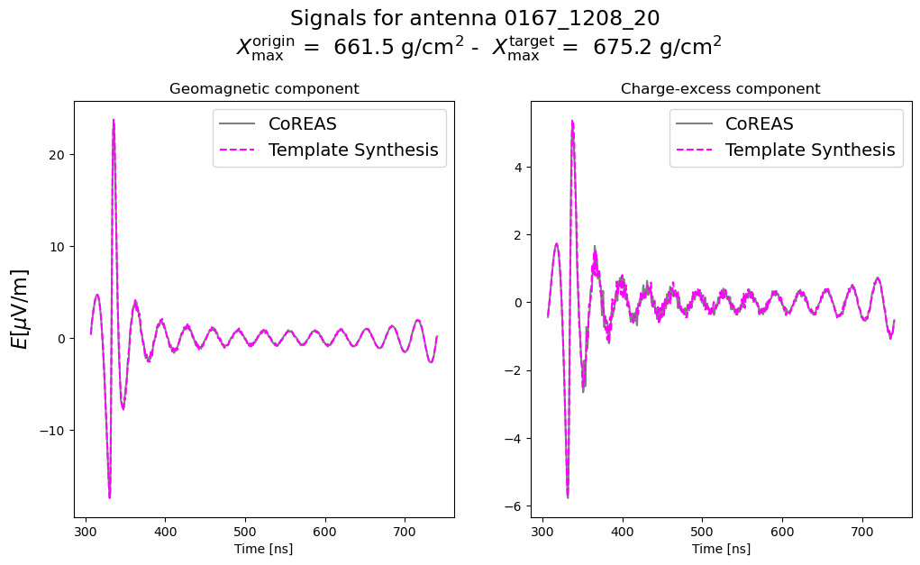
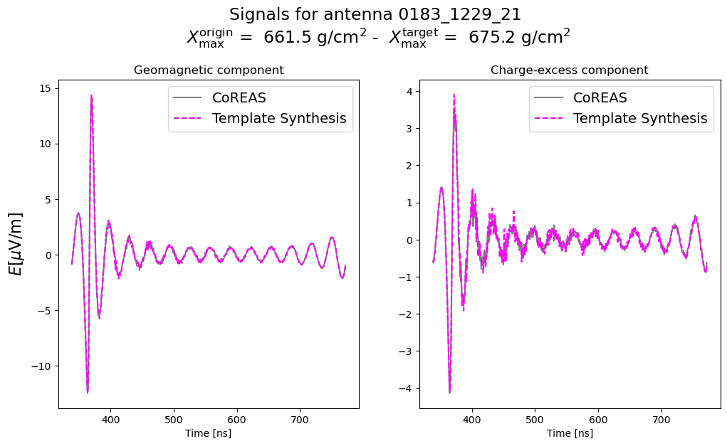
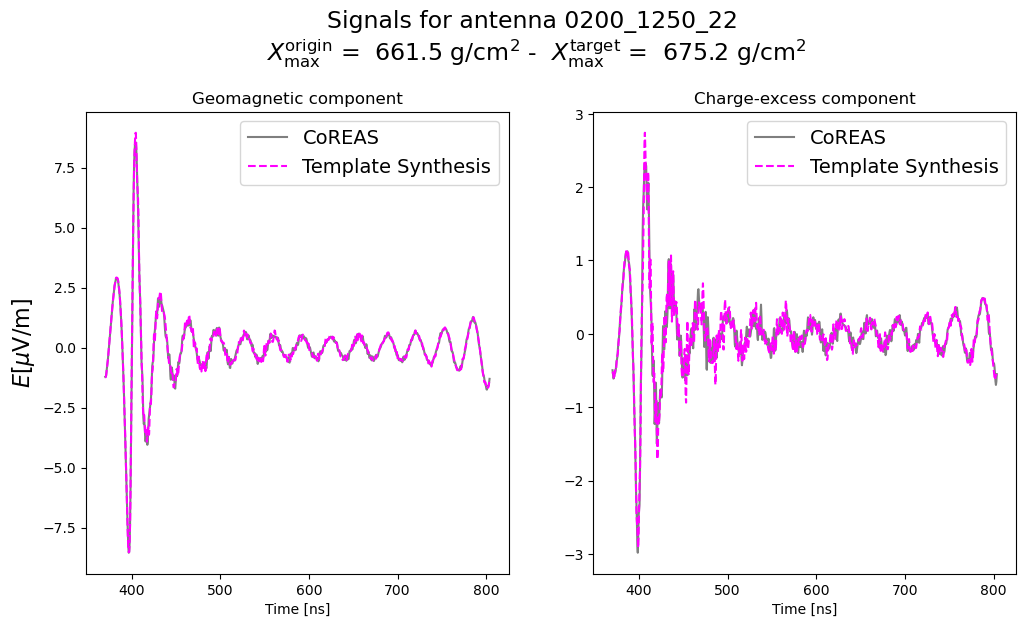
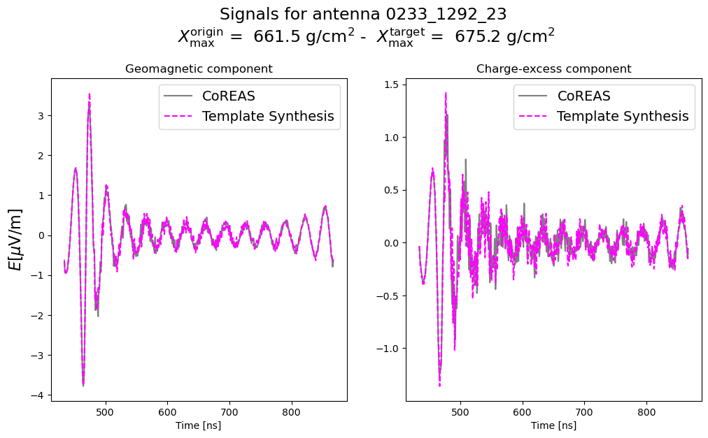
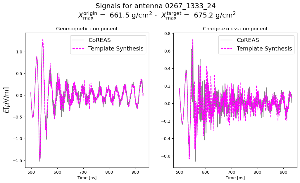
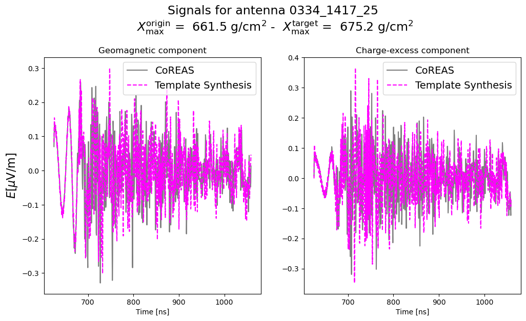
for ant_idx, ant_name in enumerate(ant_names):
    geo_target, ce_target, start_target = target.get_trace_geoce(ant_name, bandpass=[30 * units.MHz, 500 * units.MHz], return_start_time=True)

    target_time = np.arange(geo_target.shape[1]) * target.delta_t + start_target[0]

    fig, ax = plt.subplots(1, 2, figsize=(12, 6))
    ax = ax.flatten()

    ax[0].plot(
        target_time / units.ns,
        np.sum(geo_target, axis=0) / (units.microvolt / units.m),
        c='k', label='CoREAS',
        alpha=0.5
    )
    ax[1].plot(
        target_time / units.ns,
        np.sum(ce_target, axis=0) / (units.microvolt / units.m),
        c='k', label='CoREAS',
        alpha=0.5
    )

    ax[0].plot(
        origin_time[ant_idx],
        total_geo_synth[ant_idx] / (units.microvolt / units.m),
        '--',
        c='magenta', label='Template Synthesis',
    )
    ax[1].plot(
        origin_time[ant_idx],
        total_ce_synth[ant_idx] / (units.microvolt / units.m),
        '--',
        c='magenta', label='Template Synthesis',
    )

    ax[0].set_ylabel(r'$E [\mu \mathrm{V}/\mathrm{m}]$', size=16)
    ax[0].set_xlabel('Time [ns]')
    ax[1].set_xlabel('Time [ns]')

    ax[0].legend(fontsize=14)
    ax[1].legend(fontsize=14)

    ax[0].set_title('Geomagnetic component')
    ax[1].set_title('Charge-excess component')

    fig.suptitle(f'Signals for antenna {ant_name} \n'
                 r'$X^{\mathrm{origin}}_{\mathrm{max}}$ = ' + f' {origin.xmax:.1f} ' + r'$\mathrm{g}/\mathrm{cm}^2$' + ' - '
                 r' $X^{\mathrm{target}}_{\mathrm{max}}$ = ' + f' {target.xmax:.1f} ' + r'$\mathrm{g}/\mathrm{cm}^2$'
                 '\n', y=1.05, size=17)
/tmp/ipykernel_220006/3654000733.py:6: RuntimeWarning: More than 20 figures have been opened. Figures created through the pyplot interface (matplotlib.pyplot.figure) are retained until explicitly closed and may consume too much memory. (To control this warning, see the rcParam figure.max_open_warning). Consider using matplotlib.pyplot.close().
  fig, ax = plt.subplots(1, 2, figsize=(12, 6))
Saving and loading templates
This can be done by giving a save and load path, which will store all relevant quantities in a HDF5 file.
If template_file=None, then the name of the origin shower
(SIMXXXXXX) will be used.
synthesis.save_template(
    save_dir='./',  # path to where you want to save the template
    template_file = './template_test.hdf5'  # optional: specify the file name
)
0
To load the template, only the path to the template needs to be provided.
If the origin shower uses GDAS atmospheres, then the path to the relevant GDAS file needs to be additionally provided.
synthesis.load_template(
    file_path='./template_test.hdf5',
    gdas_file=None
)
0