Synthesising a single shower¶

While other examples show how to synthesise many target showers with a large origin library, here we show a more minimal example of how to synthesise a single shower from a single origin shower.

This can be useful if you want to: - test if the synthesis works at a basic level - if you have a single origin shower at hand - want to understand SMIET at a more basic level - dont want to use the library, but manually generated origin showers

from smiet import SMIETRun, units
import numpy as np
import matplotlib.pyplot as plt  # for plotting

Paths¶

The only required path here is the path to the origin shower that you want to synthesise with.

path_to_origin_shower = "/home/kwatanabe/Projects/radio-ift/radio_resources/template_synthesis/origin_library/base/SIM000000.hdf5"

As before, one needs to set the site, which configures the magnetic field and frequency range used in SMIET.

smiet_runner = SMIETRun(site='base', backend='numpy')

To then synthesise a single shower, the following must be provided:

• the path to the origin shower (including the hdf5 file), generated for sliced showers

• the longitudinal profile to use for synthesis

• the grammage array

• the target zenith angle

Additionally, the azimuth angle and the core can also be set separately. Note that the Xmax and Nmax used in the synthesis is automatically set by grammages[argmax(profile)] and max(profile).

This function will: - Initialize a sliced shower instance - make a template with that - generate a basic shower object and set the provided parameters - map the template to get the synthesised traces in the geomagnetic and charge-excess component

The traces that follow the same antenna positions as the origin shower will be returned (in GEO / CE polarization), as well as the time axes for the shower.

NOTE: there are no rigorous checks if the Xmax or zenith of the origin are close to that of the target. Be aware that the performance degrades if the origin Xmax / zenith is far from the target shower.

def gaisser_hillas_function(x, nmax, x0, xmax, lmbda):
    power = (xmax - x0) / lmbda

    result = np.nan_to_num(np.where((x - x0) >= 0, (
        nmax
        * ((x - x0) / (xmax - x0)) ** power
        * np.exp((xmax - x) / lmbda)
    ), 0.0))
    return result

grammage_grid = np.linspace(0, 1100, 200)
long_profile = gaisser_hillas_function(grammage_grid, nmax=1e9, x0=0, xmax=700, lmbda=70)

synth_geo, synth_ce, times = smiet_runner.synthesize_with_single_origin(
    origin_shower_path = path_to_origin_shower,
    target_long=long_profile,
    target_grammage = grammage_grid,
    target_zenith = 0 # in degrees
)

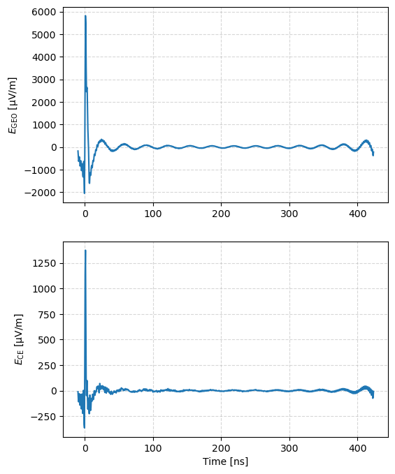
Plotting the results¶

ant_idx = 1  # choose an antenna index to plot

fig, ax = plt.subplots(2,1, figsize=(6,8))

ax[0].plot(times[ant_idx, :] / units.ns, synth_geo[ant_idx,:] / (units.micro  * units.volt / units.m))
ax[1].plot(times[ant_idx, :] / units.ns, synth_ce[ant_idx,:] / (units.micro  * units.volt / units.m))
ax[1].set_xlabel("Time [ns]")
ax[0].set_ylabel(r"$E_\mathrm{GEO}$ [μV/m]")
ax[1].set_ylabel(r"$E_\mathrm{CE}$ [μV/m]")

# ax[0].set_title(f"Time traces at {ant_name}")
ax[0].grid(True, which="both", ls="--", alpha=0.5)
ax[1].grid(True, which="both", ls="--", alpha=0.5)