Running SMIET with User-Generated Target Showers
This is an example notebook on how to run SMIET using the main functionality SMIETRun.
For most intensive purposes, using this module is sufficient.
from smiet import SMIETRun, units
import numpy as np

import matplotlib.pyplot as plt  # for plotting routines
import logging
logger = logging.getLogger('smiet')

# Set the top-level logger to DEBUG
logger.setLevel(logging.WARNING)
Setting up paths
For this version, the following paths are required:
the path to where the templates are loaded
path_to_templates = "/home/kwatanabe/Projects/radio-ift/radio_resources/template_synthesis/origin_library/templates"
Initializing the object
The SMIETRun object is initialized with the following: - site : the site in which we perform the synthesis. Currently, base, lofar, and auger are supported, with more to come! - backend : this allows you to choose whether to run smiet with the numpy backend (recommended!) or with jax (disabled for now, as it has not yet been tested).
Under the hood, the numpy or jax version of smiet will be loaded with the given site parameters fixed.
smiet_runner = SMIETRun(
    site="base", backend="numpy"
)
(Optional) : Generate the template library
Once you have generated simulations from the origin shower library, it is most convenient for you to generate a template library, which can then be loaded / unloaded with ease later on.
The template libraries themselves will be provided for the users to download, making this step optional. However, if you have generated your own origin shower library, then this step is necessary.
To run this, provide the repository in which the origin library (the
hdf5 files) are located in origin_shower_repo, and the repository in
which you want to store the templates in template_repo. The
directory structure will automatically be built to be separated by xmax
and zenith bins, set by the user.
NOTE : the generation of the templates can take a while. Take a cup of coffee and chat with your colleagues while this is running :D
# smiet_runner.generate_templates(
#     origin_shower_repo = "/home/kwatanabe/Projects/radio-ift/radio_resources/template_synthesis/origin_library/base",
#     template_repo = "/home/kwatanabe/Projects/radio-ift/radio_resources/template_synthesis/origin_library/templates"
# )
Loading the templates
Here, all necessary templates which will be used for the analysis can be
loaded. To load the templates, provide the repository in which the
templates are located in template_repo.
We give the option to provide a range of xmax and zenith values in which
the templates should be loaded, to avoid load unnecessary values of Xmax
or zenith angles. This can be performed by giving: - a tuple of
(xmax_min, xmax_max) in xmax_range - a tuple of (zenith_min,
zenith_max) in zenith_range If nothing is provided, then the full
range of available templates will be loaded instead.
Additionally, with the randomize argument set to True, one of the
simulated origin showers from the configuration will be selected at
random. If set to False, the first one will always be selected.
# load templates
smiet_runner.load_templates(
    template_repo = path_to_templates,
    xmax_range = (700, 1000),
    zenith_range = (36, 40),
    randomize = False
)
Note that the properties of the origin showers can be extracted using
smiet_runner.origin_properties().
Alternatively, the xmax and zenith values for the origin shower are
given by smiet_runner.origin_xmaxs and
smiet_runner.origin_zeniths respectively.
print(smiet_runner.origin_xmaxs, smiet_runner.origin_zeniths)
[ 697.21 704.82 751.53 804.07 880.63 889.21 1001.7 1006.4 ] [36. 39. 39. 36. 36. 39. 39. 36.]
Generating target showers
The target showers are the showers that will be synthesized with SMIET. These can be set in two ways:
from user-generated longitudinal profiles
from a set of simulated showers from CoREAS
We will show how to generate target showers manually here, and show its usability with CoREAS showers in another example notebook.
Here, we define the Gaisser-Hillas function for the longitudinal profile. In the future, a package that can self-consistently generate various kinds of longitudinal profiles will be implemented, removing the need for this function.
def gaisser_hillas_function(x, nmax, x0, xmax, lmbda):
    power = (xmax - x0) / lmbda

    result = np.nan_to_num(np.where((x - x0) >= 0, (
        nmax
        * ((x - x0) / (xmax - x0)) ** power
        * np.exp((xmax - x) / lmbda)
    ), 0.0))
    return result
The inputs require the following: - a grid of grammage. This need not be the same as the origin shower - a list of longitudinal profiles generated with the same grammage grid - an array of zenith angles
Optionally, one can: - provide an array of azimuth angles - provide an array of cores
# now generate some target longitudinal profiles
target_xmaxs = np.array([800, 710.0])
target_zeniths = np.deg2rad(np.array([37.5, 38.5]))

grammage_grid = np.linspace(0, 1100, 200)
long_profs = []
for xmax in target_xmaxs:
    long_profs.append( gaisser_hillas_function(
        grammage_grid, nmax = 1e8, x0 = 0.0, xmax=xmax, lmbda = 70.0
    ))
smiet_runner.generate_target_showers(
    target_grammage = grammage_grid,
    target_longs = long_profs,
    target_zeniths = target_zeniths
)
Similar to the origin showers, the properties of the target showers can
be extracted using smiet_runner.target_properties().
The xmax and zenith values for the target showers are given by
smiet_runner.target_xmaxs and smiet_runner.target_zeniths
respectively.
print(smiet_runner.target_xmaxs, smiet_runner.target_zeniths)
[800.00000115 709.9999972 ] [37.5 38.5]
Synthesizing showers
The main code here is the synthesis of the showers. This will (for each target shower):
find the origin shower with the closest Xmax values (larger or smaller) and zenith angle (smaller)
Synthesise the shower in the vx(vxB) component with the origin shower with Xmax < target Xmax
Reconstruct the star-shape pattern from the synthesized traces
Depending on the selected options, additional features can be enabled: -
interpolation : if True, then synthesis with origin shower > target
Xmax will additionally performed, and the resulting synthesised trace
will be a weighted result between both traces - slices : If True,
then traces from all slices will be saved. Otherwise only the trace at
the ground will be stored.
The synthesised traces are stored as class objects via
smiet_runner.synth_traces.
Note: the synthesis scales with the number of showers you want to synthesise. Each synthesis takes ~ 10 seconds.
smiet_runner.synthesize_showers(slices=True, interpolation=True)
[93m2025-11-25 23:34:20 - WARNING - smiet.core.SMIETRun - synthesize_showers - Synthesis with slices=True is enabled. Setting interpolation=False since it does not work with interpolated synthesis.[0m
Accessing synthesized quantities
To extract the synthesized showers, we can either: - get the traces - get the spectrum - or get the fluence
The traces and spectra is extracted for a given target xmax and zenith
angle, which can be indexed through smiet_runner.target_xmaxs and
smiet_runner.target_zeniths. The following options are additionally
available: - ant_name : a specific antenna label, following the
names from smiet_runner.antenna_labels can be set to get a single
antenna position. Setting this to None will give all antennas. -
geoce : If true, then the geomagnetic / charge-excess polarisation
will be returned, otherwise the vxB / vx(vxB) polarisation will be
returned instead. - slice_grammage : the traces at a specific slice
can be returned if slices=True is set when synthesising the showers.
If None, then only the one at ground will be stored.
ant_name = "ant_r75_phi315" # an example. the antennas are labelled as `ant_r<radius>_phi<angle in degree>`.
target_xmax_to_get, target_zeniths_to_get = smiet_runner.target_xmaxs[0], smiet_runner.target_zeniths[0]
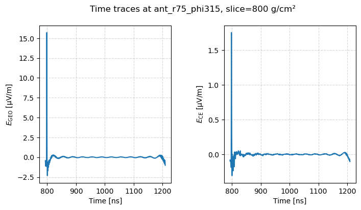
Traces
The get_traces function returns: - traces : in shape of (Npol, Nant,
Nsamples) if ant_name = None, otherwise (Npol, Nsamples) - times :
in shape of (Nant, Nsamples) if ant_name = None, otherwise
(Nsamples) - antenna positions in the shower plane, in shape of (Nant)
or () if ant_name != None.
Note that the units module is necessary to appropriately convert to
the desired units.
traces_geoce, times, _ = smiet_runner.get_traces(
    xmax=target_xmax_to_get,
    zenith=target_zeniths_to_get,
    ant_name=ant_name,
    geoce=True,
    slice_grammage=800,
)
fig, ax = plt.subplots(1,2, figsize=(8,4), gridspec_kw={"wspace":0.4})
ax[0].plot(times[:] / units.ns, traces_geoce[0,:] / (units.micro  * units.volt / units.m))
ax[1].plot(times[:] / units.ns, traces_geoce[1,:] / (units.micro  * units.volt / units.m))
ax[0].set_xlabel("Time [ns]")
ax[1].set_xlabel("Time [ns]")
ax[0].set_ylabel(r"$E_\mathrm{GEO}$ [μV/m]")
ax[1].set_ylabel(r"$E_\mathrm{CE}$ [μV/m]")

fig.suptitle(f"Time traces at {ant_name}, slice=800 g/cm²")
ax[0].grid(True, which="both", ls="--", alpha=0.5)
ax[1].grid(True, which="both", ls="--", alpha=0.5)
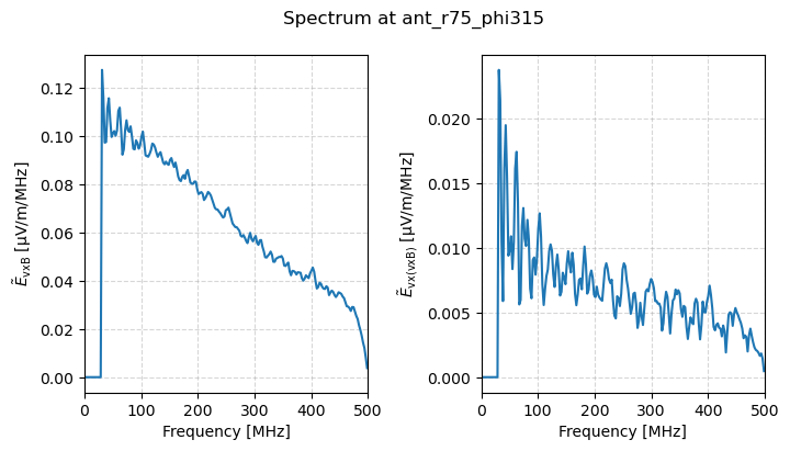
Spectra
spectrum : the real-component of the spectrum, both amplitude and phase (traces + FFT with
orthonormalisation) in shapes of (Npol, Nant, Nfreqs) or (Npol, Nfreqs)frequencies : the frequency grid, in internal units with shape of (Nfreqs, )
spect_geoce, freq = smiet_runner.get_spectrum(
    xmax=target_xmax_to_get,
    zenith=target_zeniths_to_get,
    ant_name=ant_name,
    geoce=False,
    slice_grammage=None,
)
fig, ax = plt.subplots(1,2, figsize=(8,4), gridspec_kw={"wspace":0.4})
ax[0].plot(freq / units.MHz, np.abs(spect_geoce[0,:]) / (units.micro  * units.volt / units.m / units.MHz))
ax[1].plot(freq / units.MHz, np.abs(spect_geoce[1,:]) / (units.micro  * units.volt / units.m / units.MHz))
ax[0].set_xlabel("Frequency [MHz]")
ax[1].set_xlabel("Frequency [MHz]")
ax[0].set_xlim(0, 500)
ax[1].set_xlim(0, 500)
ax[0].set_ylabel(r"$\tilde{E}_\mathrm{vxB}$ [μV/m/MHz]")
ax[1].set_ylabel(r"$\tilde{E}_\mathrm{vx(vxB)}$ [μV/m/MHz]")

fig.suptitle(f"Spectrum at {ant_name}")
ax[0].grid(True, which="both", ls="--", alpha=0.5)
ax[1].grid(True, which="both", ls="--", alpha=0.5)
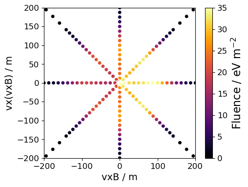
Fluence
The energy fluence (in units of eV/m^2) can additionally be extracted with similar arguments. The antenna positions in the shower plane are also returned for easy access for e.g. scatter plots.
fluences, ant_pos = smiet_runner.get_fluence(
    xmax=target_xmax_to_get,
    zenith=target_zeniths_to_get,
    geoce=False,
    slice_grammage=None,
)
fig, ax = plt.subplots(1,1, figsize=(5,4))
sc = ax.scatter(
    ant_pos[:, 0], ant_pos[:, 1],
    c=fluences,
    cmap='inferno',
    edgecolor='white',
    alpha=1.0,
    vmin=0,
    vmax=35  # modify as needed
)

ax.set_xlabel("vxB / m", fontsize=14)
ax.set_ylabel("vx(vxB) / m", fontsize=14)

ax.set_xlim(-200, 200)
ax.set_ylim(-200, 200)

ax.tick_params(axis='both', which='major', labelsize=12)

cbar = fig.colorbar(sc, ax=ax)
cbar.ax.set_ylabel("Fluence / eV m$^{-2}$", fontsize=16)
cbar.ax.tick_params(labelsize=12)