Using the JAX version¶

As mentioned in the README, there also exists a version in JAX, which is a high-performant language framework in Python that supports JIT-compilation, GPU/TPU accelerated framework, automatic differentiation, and parallelization.

This is implemented to be applied in the context of NIFTy. However, it can also be used to synthesise traces normally. This is generally not recommended, however, as:

For most general cases, the numpy

version is sufficient in terms of performance,

it can be annoying to

install jax in your machine, especially if you want to use the GPU features

there may be memory issues related to it for large origin showers (fix in progress!)
some features may not be directly available.

Nevertheless, we provide the user with a way to run and compare the JAX version with the numpy version here.

import jax

# IMPORTANT! set the device and enable x64 for precision
jax.config.update("jax_enable_x64", True)
jax.config.update("jax_platform_name", "cpu")

import jax.numpy as jnp  # numpy API from jax
import numpy as np

import matplotlib.pyplot as plt

import smiet.numpy as smiet_np
import smiet.jax as smiet_jax  # will fail if JAX is not installed

from smiet import units

Paths and setup¶

# Selections (to be put in main)
ANT_DEBUG = None
FREQ = [30, 500, 100]

# Variables
shower_path = '/home/kwatanabe/Projects/radio-ift/radio_resources/template_synthesis/origin_library/base'
shower_origin = "000100"
shower_target = "000111"

Synthesising a single origin shower from a SlicedShower with JAX¶

origin_jax = smiet_jax.SlicedShower(f'{shower_path}/SIM{shower_origin}.hdf5')
target_jax = smiet_jax.SlicedShower(f'{shower_path}/SIM{shower_target}.hdf5')

synthesis_jax = smiet_jax.TemplateSynthesis(freq_ar=FREQ)
synthesis_jax.make_template(origin_jax)
synth_geo_jax, synth_ce_jax = synthesis_jax.map_template(target_jax)

synth_dcore_jax = np.linalg.norm(synthesis_jax.antenna_information["position_showerplane"][:,:2], axis=1)

Get the target CoREAS slice traces from the JAX version¶

geo_target, ce_target = target_jax.get_traces_geoce()  # already bandpass filtered to [30, 500] MHz
geo_target = np.sum(geo_target, axis=-1)
ce_target = np.sum(ce_target, axis=-1)

Do the same thing for NumPy¶

origin_np = smiet_np.SlicedShower(f'{shower_path}/SIM{shower_origin}.hdf5')
target_np = smiet_np.SlicedShower(f'{shower_path}/SIM{shower_target}.hdf5')

synthesis_np = smiet_np.TemplateSynthesis(freq_ar=FREQ)
synthesis_np.make_template(origin_np)
synth_geo_np, synth_ce_np = synthesis_np.map_template(target_np)

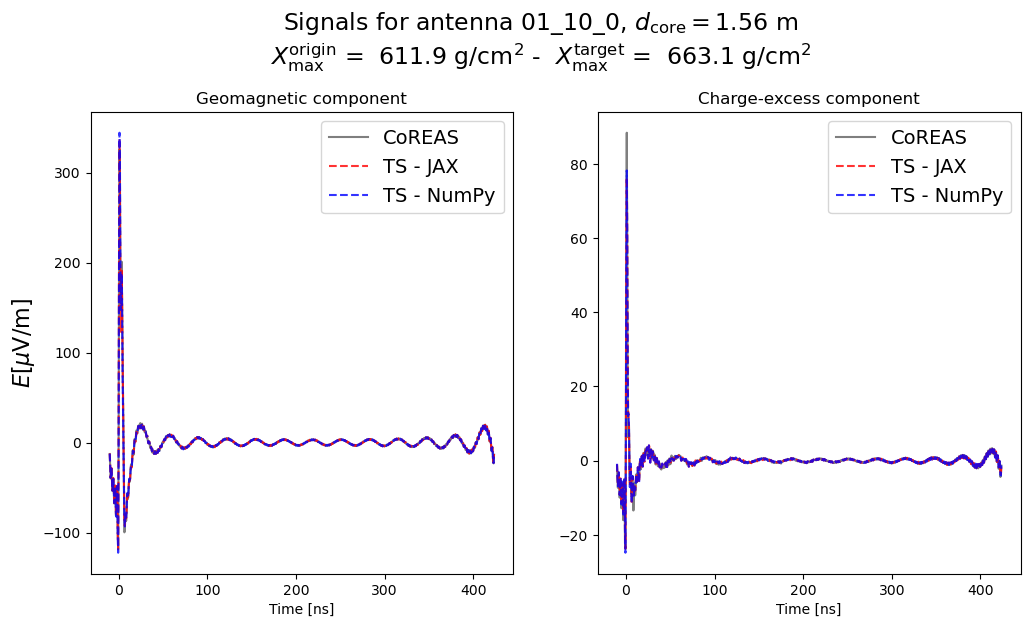
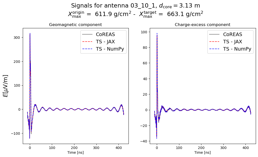
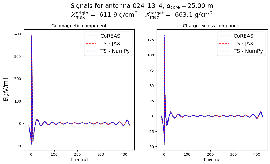
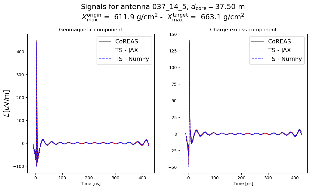
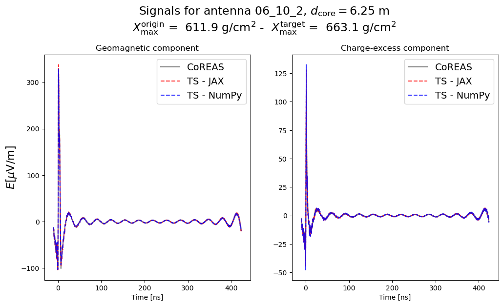
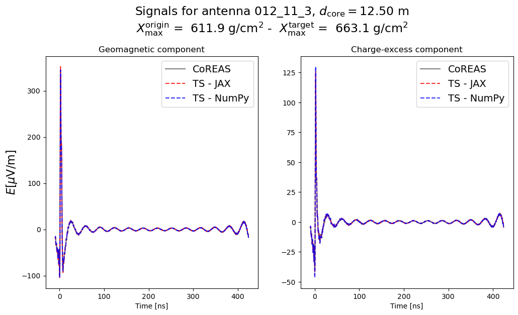
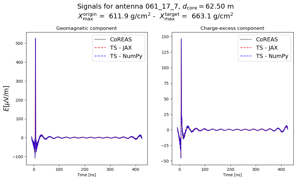
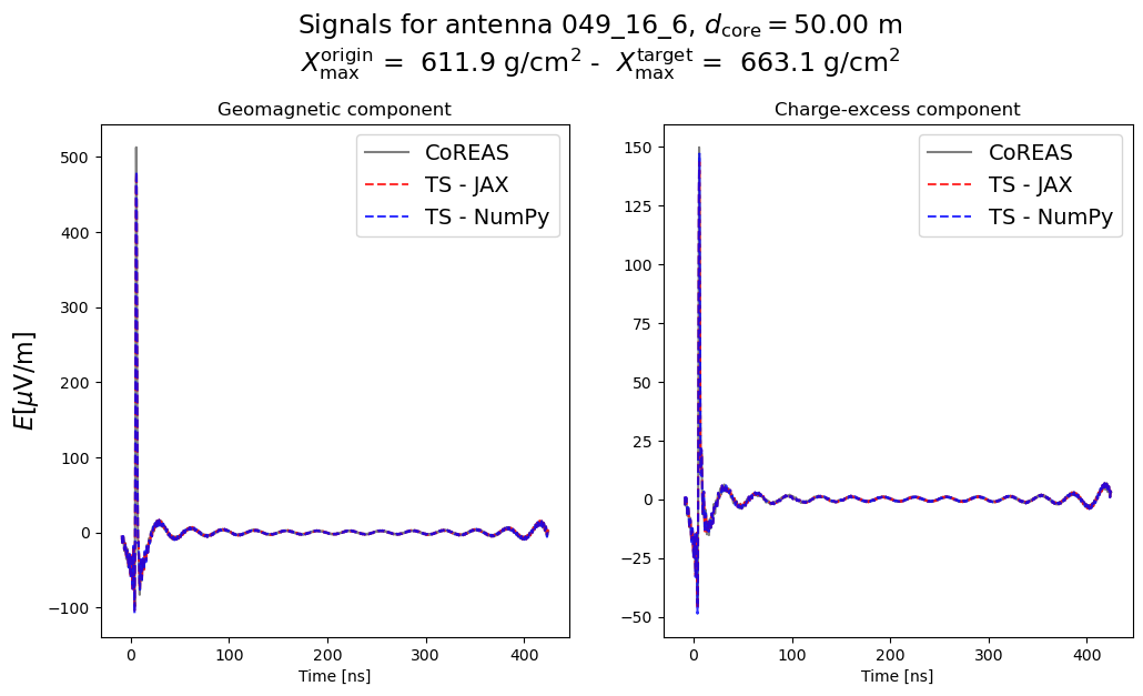
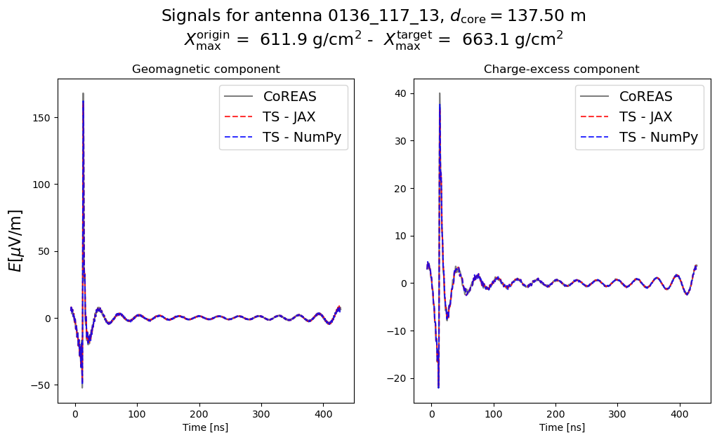
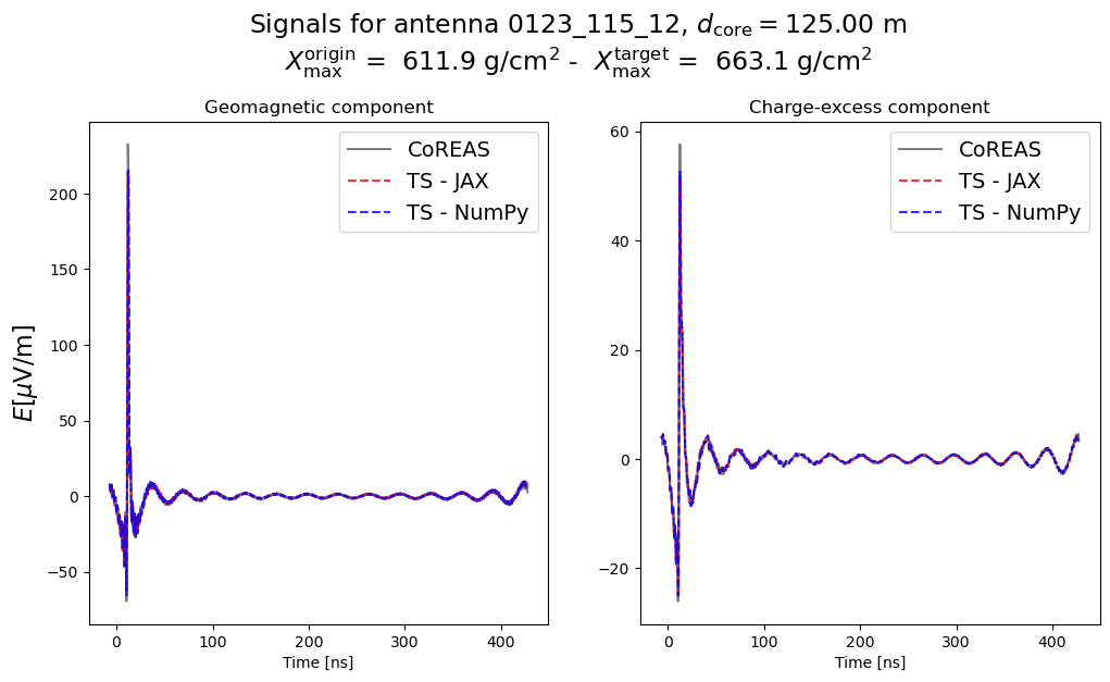
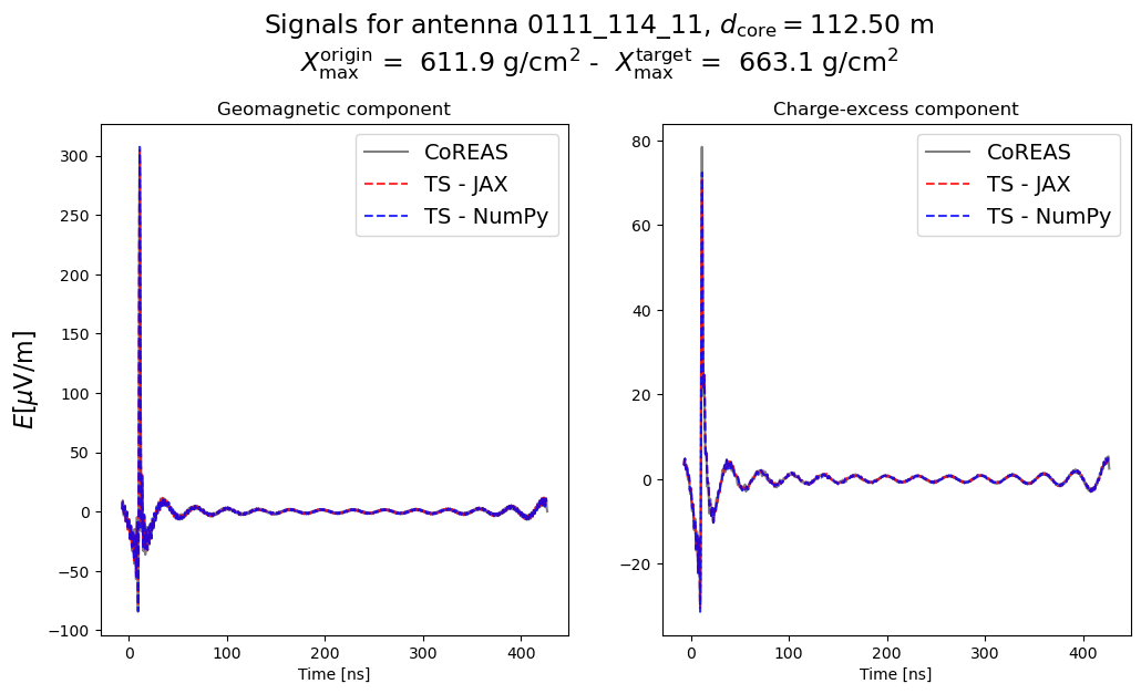
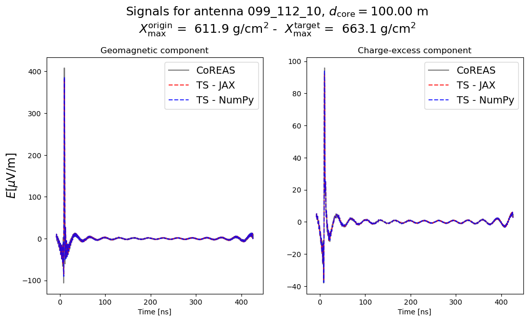
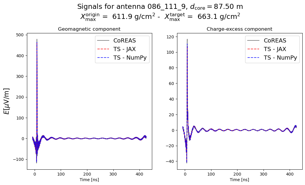
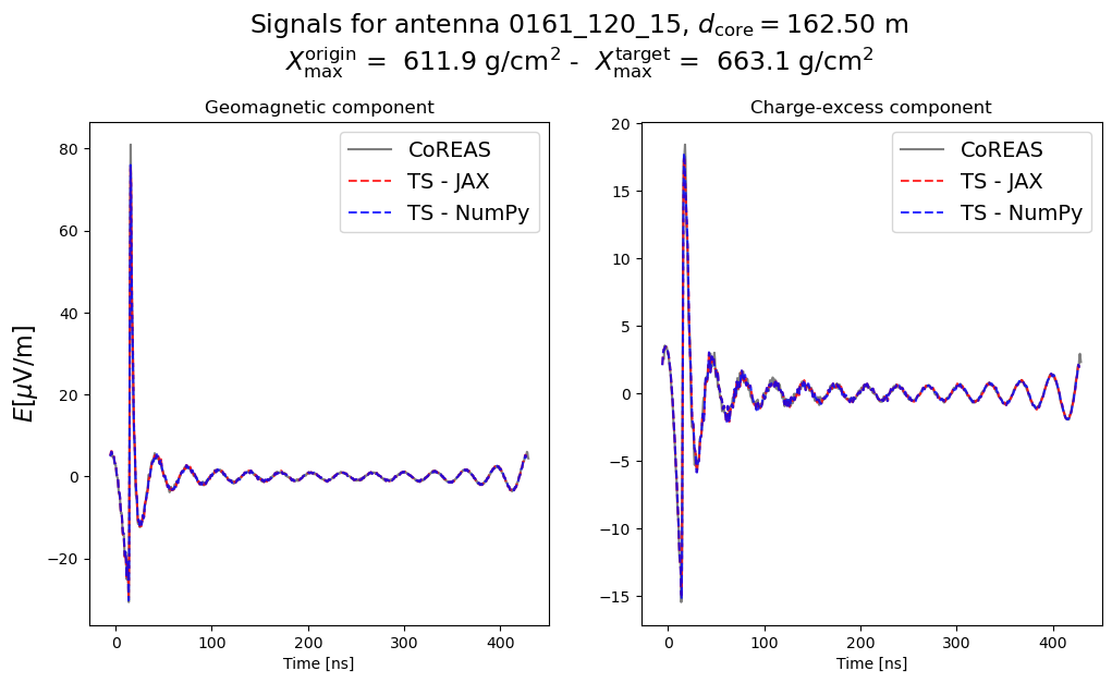
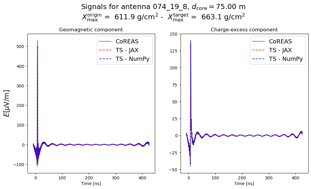
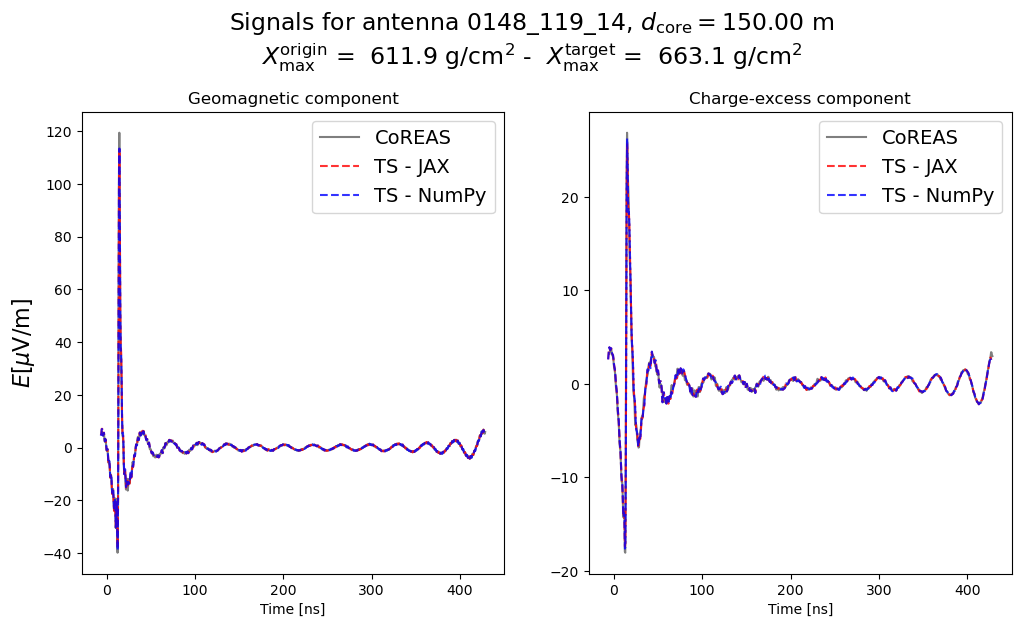
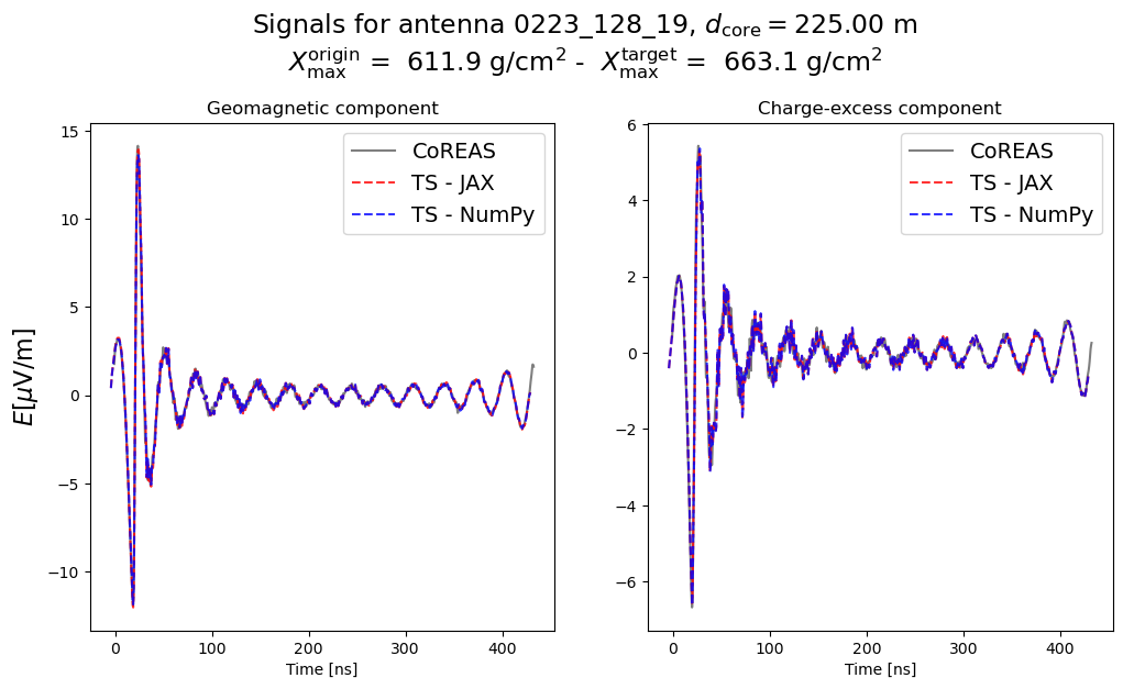
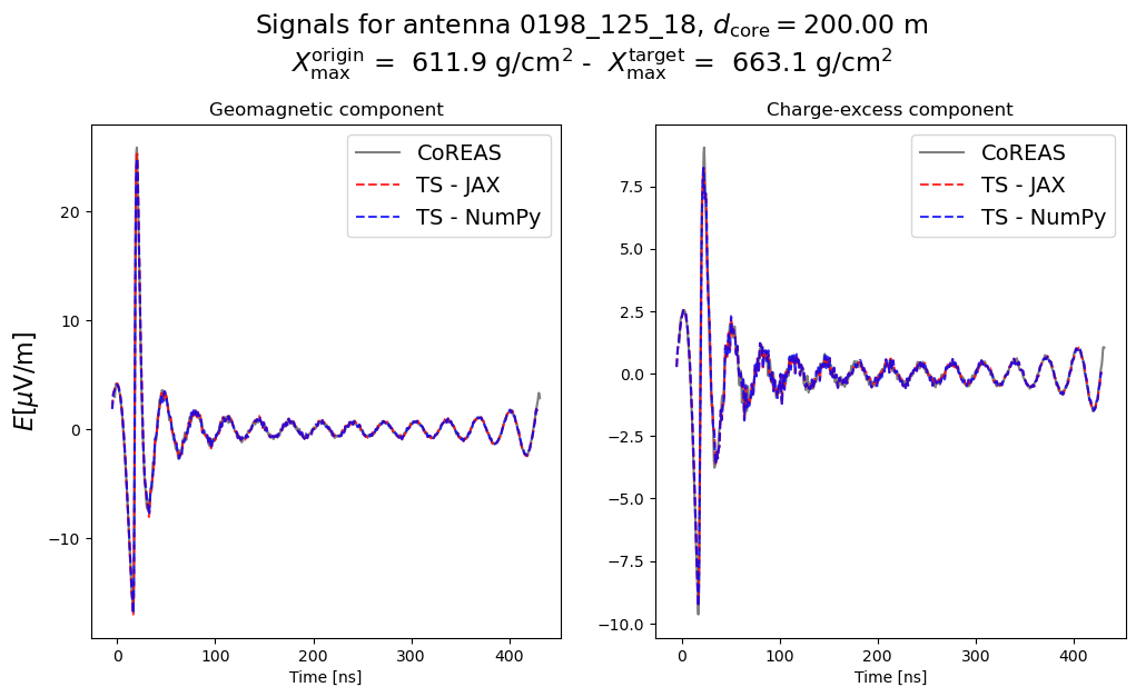
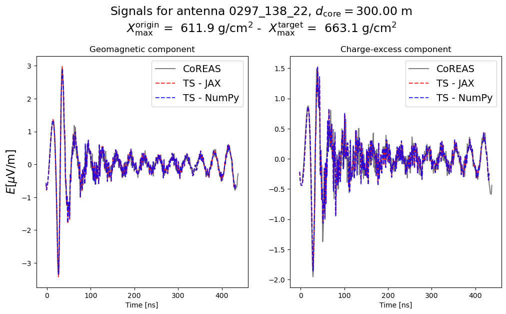
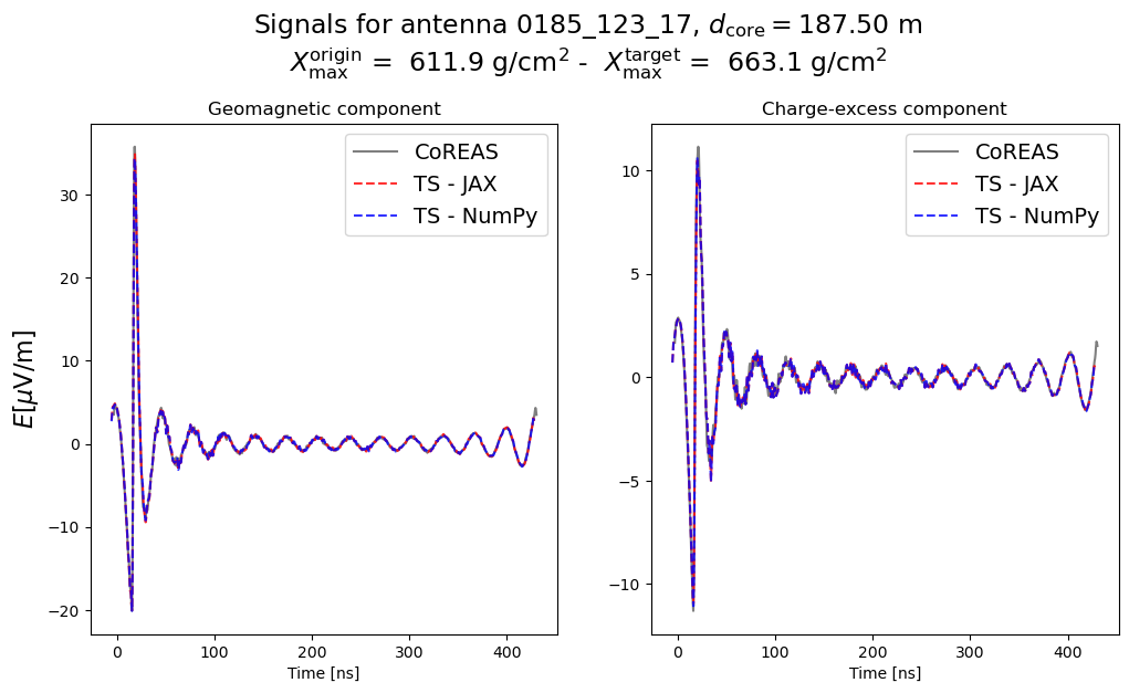
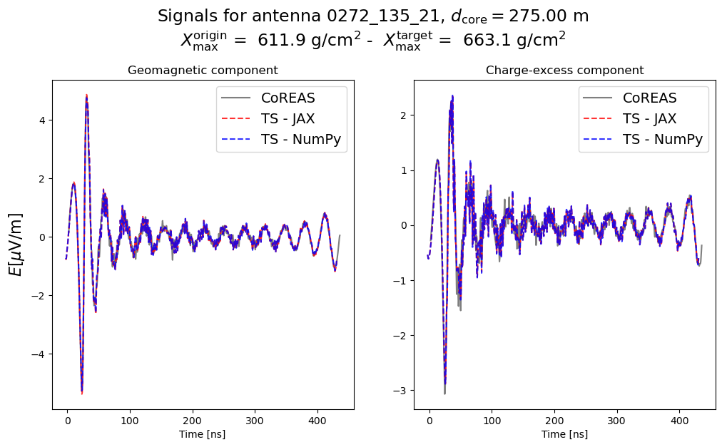
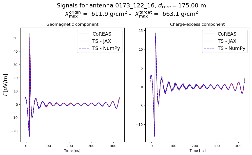
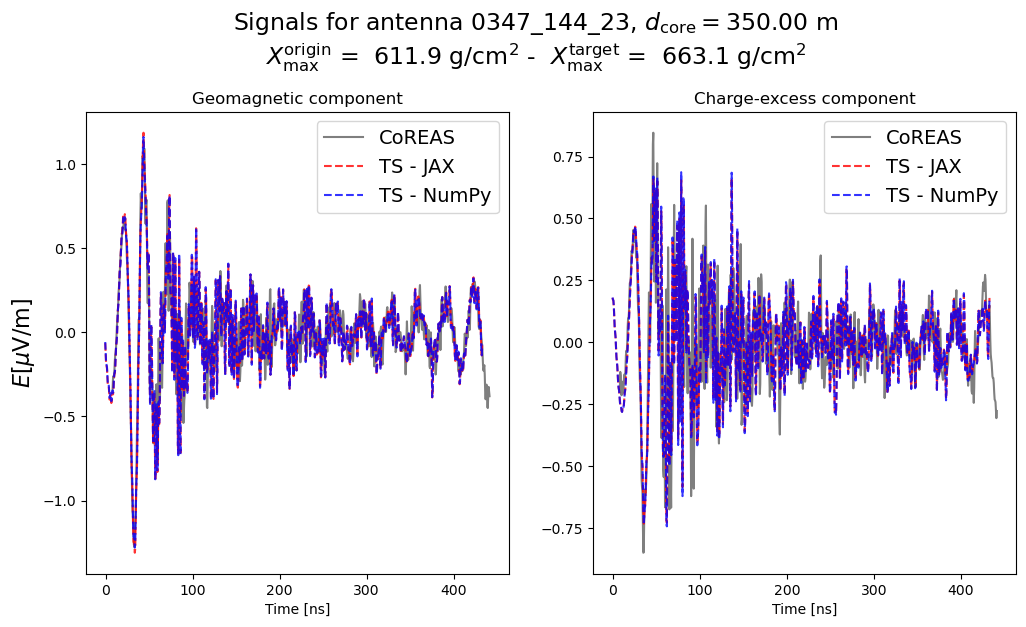
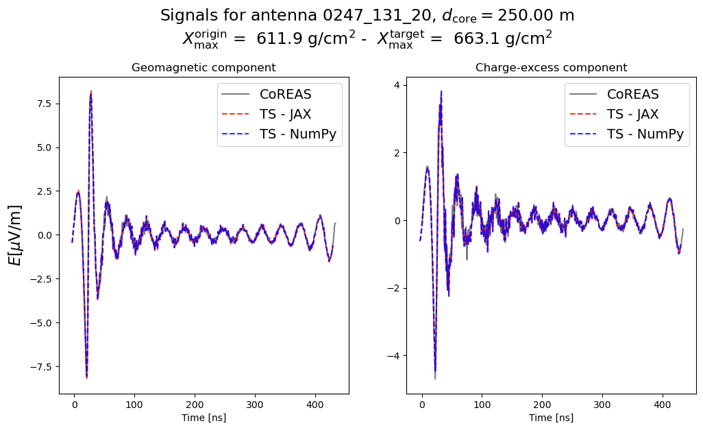
Compare both implementations¶

for ant_idx, ant_name in enumerate(synthesis_jax.get_antenna_names()):

    fig, ax = plt.subplots(1, 2, figsize=(12, 6))
    ax = ax.flatten()

    # find the antenna index comparing the distance to the core,
    # since the antenna positions may not exactly match
    ant_idx_target = np.argmin(
        np.abs(target_jax.antenna_array["dis_to_core"] - synth_dcore_jax[ant_idx])
    )

    time_axis = np.arange(geo_target.shape[1]) * target_jax.delta_t + target_jax.trace_times[ant_idx_target,0]

    ax[0].plot(
        time_axis,
        geo_target[ant_idx_target,:] / (units.microvolt / units.m),
        c='k', label='CoREAS',
        alpha=0.5
    )
    ax[1].plot(
        time_axis,
        ce_target[ant_idx_target,:] / (units.microvolt / units.m),
        c='k', label='CoREAS',
        alpha=0.5
    )

    ax[0].plot(
        synthesis_jax.get_time_axis()[ant_idx],
        synth_geo_jax[ant_idx] / (units.microvolt / units.m),
        '--',
        c='r', label='TS - JAX',
        alpha=0.8
    )
    ax[1].plot(
        synthesis_jax.get_time_axis()[ant_idx],
        synth_ce_jax[ant_idx] / (units.microvolt / units.m),
        '--',
        c='r', label='TS - JAX',
        alpha=0.8
    )

    # find the antenna name in the numpy version, since the indices
    # may not match
    ant_idx_np = list(synthesis_np.get_antenna_names()).index(ant_name)

    ax[0].plot(
        synthesis_np.get_time_axis()[ant_idx_np],
        synth_geo_np[ant_idx_np] / (units.microvolt / units.m),
        '--',
        c='b', label='TS - NumPy',
        alpha = 0.8
    )
    ax[1].plot(
        synthesis_np.get_time_axis()[ant_idx_np],
        synth_ce_np[ant_idx_np] / (units.microvolt / units.m),
        '--',
        c='b', label='TS - NumPy',
        alpha = 0.8
    )

    # ax[0].set_xlim([-10, 100])
    # ax[1].set_xlim([-10, 100])

    ax[0].set_ylabel(r'$E [\mu \mathrm{V}/\mathrm{m}]$', size=16)
    ax[0].set_xlabel('Time [ns]')
    ax[1].set_xlabel('Time [ns]')

    ax[0].legend(fontsize=14)
    ax[1].legend(fontsize=14)

    ax[0].set_title('Geomagnetic component')
    ax[1].set_title('Charge-excess component')

    fig.suptitle(fr'Signals for antenna {ant_name}, $d_\mathrm{{core}} = {target_jax.antenna_array["dis_to_core"][ant_idx_target]:.2f}$ m' + '\n'
                 r'$X^{\mathrm{origin}}_{\mathrm{max}}$ = ' + f' {origin_jax.xmax:.1f} ' + r'$\mathrm{g}/\mathrm{cm}^2$' + ' - '
                 r' $X^{\mathrm{target}}_{\mathrm{max}}$ = ' + f' {target_jax.xmax:.1f} ' + r'$\mathrm{g}/\mathrm{cm}^2$'
                 '\n', y=1.05, size=17)

/tmp/ipykernel_225867/4190965798.py:3: RuntimeWarning: More than 20 figures have been opened. Figures created through the pyplot interface (matplotlib.pyplot.figure) are retained until explicitly closed and may consume too much memory. (To control this warning, see the rcParam figure.max_open_warning). Consider using matplotlib.pyplot.close().
  fig, ax = plt.subplots(1, 2, figsize=(12, 6))

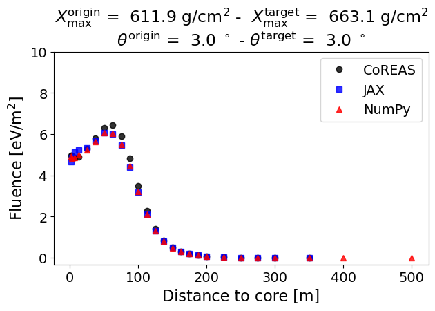
Comparing the fluence distribution¶

def get_fluence(traces, delta_t):
    """Calculate fluence from traces.

    Args:
        traces (ndarray): shape (n_pol, n_antennas, n_times)
        delta_t (float): time step in nanoseconds

    Returns:
        ndarray: fluence for each antenna, shape (n_antennas,)
    """
    conversion_factor_integrated_signal = 2.65441729e-3 * 6.24150934e18  # V**2/m**2 * s -> J/m**2 -> eV/m**2
    fluence = jnp.sum(traces**2, axis=(0,2)) * delta_t / units.s * conversion_factor_integrated_signal

    return fluence

target_traces = np.array([geo_target, ce_target])
synth_traces_jax = np.squeeze(np.array([synth_geo_jax, synth_ce_jax]))
synth_traces_np = np.squeeze(np.array([synth_geo_np, synth_ce_np]))

# get the distance to the core
synth_dcore_jax = np.linalg.norm(synthesis_jax.antenna_information['position_showerplane'][:,:2], axis=1)
synth_dcore_np = np.linalg.norm(synthesis_np.antenna_information["position_showerplane"][:,:2], axis=1)

fig, ax = plt.subplots(figsize=(7,4))

ax.plot(
    target_jax.antenna_array['dis_to_core'] / units.m,
    get_fluence(target_traces, delta_t = target_jax.delta_t / units.ns) / (units.eV / units.m**2),
    'o',
    label='CoREAS',
    alpha=0.8,
    ms=6,
    color='k',
    lw=2
)

ax.plot(
    synth_dcore_jax / units.m,
    get_fluence(synth_traces_jax, delta_t = synthesis_jax.delta_t / units.ns) / (units.eV / units.m**2),
    's',
    label='JAX',
    alpha=0.8,
    color='b',
    ms=6,
    lw=2
)

ax.plot(
    synth_dcore_np / units.m,
    get_fluence(synth_traces_np, delta_t = synthesis_np.delta_t / units.ns) / (units.eV / units.m**2),
    '^',
    label='NumPy',
    alpha=0.8,
    color='r',
    ms=6,
    lw=2
)

ax.set_xlabel('Distance to core [m]', size=16)
ax.set_ylabel(r'Fluence [$\mathrm{eV}/\mathrm{m}^2$]', size=16)

ax.tick_params(axis='both', which='major', labelsize=14)

ax.legend(fontsize=14)

ax.set_ylim(ymax=10)
# ax.set_xlim(xmax=20)

ax.set_title(r'$X^{\mathrm{origin}}_{\mathrm{max}}$ = ' + f' {origin_np.xmax:.1f} ' + r'$\mathrm{g}/\mathrm{cm}^2$' + ' - '
                 r' $X^{\mathrm{target}}_{\mathrm{max}}$ = ' + f' {target_np.xmax:.1f} ' + r'$\mathrm{g}/\mathrm{cm}^2$' + '\n'
                 r'$\theta^{\mathrm{origin}}$ = ' + f' {np.rad2deg(origin_np.zenith):.1f} ' + r'$^\circ$' + ' - '
                 r'$\theta^{\mathrm{target}}$ = ' + f' {np.rad2deg(target_np.zenith):.1f} ' + r'$^\circ$'
                 , size=17)

Text(0.5, 1.0, '$X^{\mathrm{origin}}_{\mathrm{max}}$ =  611.9 $\mathrm{g}/\mathrm{cm}^2$ -  $X^{\mathrm{target}}_{\mathrm{max}}$ =  663.1 $\mathrm{g}/\mathrm{cm}^2$n$\theta^{\mathrm{origin}}$ =  3.0 $^\circ$ - $\theta^{\mathrm{target}}$ =  3.0 $^\circ$')